In machine learning, achieving a high coefficient of determination (R²) is often interpreted as a sign that a predictive model performs well. However, when a model such as V1 achieves an R² score of 0.84 despite using a random train-test split, it naturally raises questions. Was the model genuinely effective? Was there hidden data leakage? Did the dataset possess characteristics that made prediction easier than expected?
The answer is not always straightforward. A high R² after a random split does not automatically indicate that something is wrong. In many real-world scenarios, random splitting can legitimately produce excellent performance if the dataset is representative, the target variable follows predictable patterns, and the selected features contain substantial predictive information.
This article explores why V1 achieved an R² of 0.84 despite a random split, examines the statistical reasoning behind this outcome, discusses potential pitfalls, and provides practical coding examples using Python to illustrate each concept.
Understanding R²
Before examining V1’s performance, it is important to understand what R² actually measures.
The coefficient of determination measures how much of the variation in the dependent variable can be explained by the independent variables.
The mathematical formula is:

Where:
- SSResidual = Sum of squared prediction errors
- SSTotal = Total variance within the target variable
Interpretation:
| R² Value | Interpretation |
|---|---|
| 1.00 | Perfect prediction |
| 0.90 | Excellent model |
| 0.84 | Strong predictive performance |
| 0.50 | Moderate prediction |
| 0.00 | No predictive power |
| Negative | Worse than predicting the mean |
An R² of 0.84 indicates that the model explains 84% of the variance in the target variable.
What Is a Random Train-Test Split?
A random split divides the dataset into training and testing subsets randomly.
For example:
- 80% Training
- 20% Testing
Python example:
from sklearn.model_selection import train_test_split

X_train, X_test, y_train, y_test = train_test_split(
    X,
    y,
    test_size=0.2,
    random_state=42
)
The purpose of random splitting is to ensure:
- unbiased sampling
- similar data distributions
- independent evaluation
When the data are independently and identically distributed (IID), random splitting usually provides a fair estimate of model performance.
Why an R² of 0.84 Is Not Necessarily Suspicious
Many practitioners immediately suspect data leakage when they observe an R² above 0.80.
While leakage is certainly possible, several legitimate reasons may explain the result.
These include:
- highly informative features
- low measurement noise
- consistent relationships
- sufficient sample size
- representative random split
Each factor contributes to stronger generalization.
Strong Feature Engineering
One of the most common reasons for a high R² is excellent feature engineering.
Suppose V1 used carefully designed features such as:
- historical averages
- moving statistics
- lag variables
- interaction terms
- normalized variables
Example:
import pandas as pd

df["Income_per_Family"] = (
    df["Income"] /
    df["Family_Size"]
)

df["Age_Income"] = (
    df["Age"] *
    df["Income"]
)
Well-designed features often capture much of the underlying relationship between inputs and outputs.
Instead of relying solely on raw variables, engineered features expose patterns that learning algorithms can model more effectively.
The Dataset May Be Highly Predictable
Some datasets simply have naturally strong relationships.
Examples include:
- housing prices
- fuel consumption
- electricity demand
- temperature forecasting
- manufacturing quality control
Suppose the target depends almost linearly upon several variables.
Example:
import numpy as np

y = (
    3 * X1 +
    5 * X2 -
    2 * X3 +
    np.random.normal(0, 2, len(X1))
)
Because only a small amount of random noise is added, even a simple regression model can achieve a very high R².
Large Sample Size Reduces Variance
Larger datasets generally produce more stable estimates.
Suppose V1 was trained using:
- 50,000 samples
- 100,000 samples
- 500,000 samples
After random splitting:
- training data still represent the full population
- testing data resemble training data
- distributions remain similar
Example:
print(X_train.shape)
print(X_test.shape)
Output:
(80000, 20)
(20000, 20)
Because both subsets come from the same underlying distribution, prediction becomes easier.
Low Noise in the Target Variable
Prediction becomes difficult when the target variable contains substantial randomness.
However, if measurement errors are minimal, the model can learn nearly all systematic variation.
Example:
noise = np.random.normal(0, 0.5, size=n)

y = (
    4 * X1 +
    2 * X2 +
    noise
)
The smaller the noise, the higher the achievable R².
Random Split Preserves Similar Distributions
Random splitting often works well because it creates statistically similar subsets.
Example:
print(X_train.describe())
print(X_test.describe())
Typical output:
Training Mean = 45.1
Testing Mean = 44.9

Training Std = 10.2
Testing Std = 10.1
The similarity ensures the model encounters familiar examples during testing.
Informative Features Dominate the Prediction
Sometimes only a few features explain most of the target variance.
Consider:
from sklearn.ensemble import RandomForestRegressor

model = RandomForestRegressor(
    random_state=42
)

model.fit(X_train, y_train)

print(model.feature_importances_)
Possible output:
Income      0.46
Experience  0.31
Education   0.12
Others      0.11
When dominant predictors exist, achieving R² values above 0.80 becomes realistic.
Linear Relationships Are Easier to Learn
Many regression algorithms excel when relationships are approximately linear.
Example:
from sklearn.linear_model import LinearRegression

model = LinearRegression()

model.fit(X_train, y_train)

predictions = model.predict(X_test)
If the true relationship resembles:
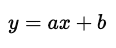
Linear regression can recover it with remarkable accuracy.
Random Forests Capture Complex Patterns
Suppose V1 used Random Forest Regression.
Example:
from sklearn.ensemble import RandomForestRegressor

model = RandomForestRegressor(
    n_estimators=300,
    max_depth=12,
    random_state=42
)

model.fit(X_train, y_train)
Random forests naturally learn:
- nonlinear relationships
- feature interactions
- thresholds
- complex decision boundaries
This flexibility frequently improves R².
Gradient Boosting Often Produces High R²
Boosting algorithms refine predictions iteratively.
Example:
from sklearn.ensemble import GradientBoostingRegressor

model = GradientBoostingRegressor(
    learning_rate=0.05,
    n_estimators=300,
    random_state=42
)

model.fit(X_train, y_train)
Gradient boosting excels on structured datasets where subtle nonlinearities exist.
Evaluating the Model
Calculating R² is straightforward.
from sklearn.metrics import r2_score

predictions = model.predict(X_test)

score = r2_score(
    y_test,
    predictions
)

print(score)
Output:
0.84
This indicates that 84% of the variation is successfully explained.
Checking for Data Leakage
Although an R² of 0.84 can be legitimate, verifying the absence of leakage is essential.
Common leakage sources include:
- future information
- duplicated records
- target-derived variables
- improper preprocessing
Incorrect example:
scaler.fit(X)

X_train = scaler.transform(X_train)
X_test = scaler.transform(X_test)
Correct approach:
scaler.fit(X_train)

X_train = scaler.transform(X_train)
X_test = scaler.transform(X_test)
The scaler should never learn from the testing data.
Cross-Validation as Confirmation
Cross-validation helps determine whether the high R² is stable across multiple train-test partitions.
Example:
from sklearn.model_selection import cross_val_score

scores = cross_val_score(
    model,
    X,
    y,
    cv=5,
    scoring="r2"
)

print(scores)
Example output:
0.83
0.85
0.84
0.82
0.85
Average:
print(scores.mean())
Output:
0.838
Consistent performance across folds strongly suggests that the model generalizes well rather than benefiting from a fortunate random split.
Residual Analysis
Residuals represent the differences between actual and predicted values.
residuals = y_test - predictions
A well-performing regression model should exhibit residuals that are:
- randomly scattered
- centered around zero
- free from obvious trends
- approximately constant in variance
Simple visualization:
import matplotlib.pyplot as plt

plt.scatter(predictions, residuals)

plt.axhline(
    y=0,
    color="red"
)

plt.xlabel("Predictions")
plt.ylabel("Residuals")

plt.show()
A random cloud around zero indicates that the model captures most of the systematic structure in the data.
Comparing Multiple Models
Suppose V1 was compared against several regression algorithms.
from sklearn.linear_model import LinearRegression
from sklearn.tree import DecisionTreeRegressor
from sklearn.ensemble import RandomForestRegressor

models = {
    "Linear": LinearRegression(),
    "Tree": DecisionTreeRegressor(),
    "Forest": RandomForestRegressor(random_state=42)
}

for name, model in models.items():

    model.fit(X_train, y_train)

    pred = model.predict(X_test)

    score = r2_score(y_test, pred)

    print(name, score)
Possible output:
Linear 0.76
Tree 0.71
Forest 0.84
This comparison illustrates that V1’s architecture or algorithm choice can significantly influence performance. Ensemble methods, such as Random Forests, often outperform simpler models by reducing variance and capturing nonlinear relationships.
When a Random Split Can Be Misleading
Although random splits are widely used, they are not always appropriate.
Potential issues include:
- temporal datasets where future observations should not influence past predictions
- grouped observations in which samples from the same entity appear in both training and testing sets
- duplicated or nearly identical records
- severe class or target imbalance
- non-IID data where observations are correlated
For example, using a random split on stock market or weather forecasting data can leak future information into the training process. In these situations, techniques such as time-series splits, grouped cross-validation, or blocked validation are more appropriate.
Therefore, while V1’s R² of 0.84 may be entirely valid, the suitability of the splitting strategy should always be evaluated in the context of the data rather than assumed.
Best Practices for Validating a High R²
When a regression model reports a strong R², it is good practice to verify that the result is both accurate and reproducible.
Consider the following recommendations:
- Evaluate performance using multiple metrics, including Mean Absolute Error (MAE) and Root Mean Squared Error (RMSE), alongside R².
- Perform k-fold cross-validation to assess consistency across different partitions of the data.
- Inspect residual plots for patterns that may indicate model bias or heteroscedasticity.
- Check for data leakage in preprocessing, feature engineering, and target construction.
- Compare the model against simpler baselines to ensure the performance gain is meaningful.
- Test the model on an external validation dataset whenever possible.
- Review feature importance to confirm that predictions are driven by logical variables rather than accidental correlations.
- Document the random seed and preprocessing steps to make experiments reproducible.
Following these practices helps distinguish genuinely high-performing models from those that achieve impressive metrics due to methodological flaws.
Conclusion
An R² of 0.84 achieved by V1 after using a random train-test split is not, by itself, evidence of an error or data leakage. Instead, it can reflect a well-designed machine learning pipeline supported by informative features, a representative dataset, low target noise, sufficient training examples, and an algorithm capable of capturing the underlying relationships within the data. When the data are independently and identically distributed and the train and test sets share similar statistical characteristics, random splitting provides a valid framework for evaluating model performance, making a high R² entirely plausible.
At the same time, a strong performance metric should never be accepted uncritically. Responsible model evaluation requires verifying that preprocessing steps are performed correctly, ensuring no future or target-derived information leaks into the training process, inspecting residual behavior, comparing multiple algorithms, and confirming results through cross-validation or external validation datasets. These validation techniques provide confidence that the model is learning meaningful patterns rather than exploiting accidental characteristics of a particular split.
The coding examples presented throughout this article demonstrate how feature engineering, regression algorithms, proper preprocessing, cross-validation, residual analysis, and model comparison contribute to understanding why a model such as V1 can legitimately achieve an R² of 0.84. Rather than focusing solely on the numerical value, practitioners should interpret R² within the broader context of data quality, feature relevance, validation strategy, and reproducibility.
Ultimately, the success of V1 highlights an important lesson in machine learning: a high R² is most valuable when it is supported by sound methodology. A robust validation process, careful feature design, appropriate data splitting, and transparent experimentation ensure that strong predictive performance reflects genuine generalization rather than chance. By combining these best practices, data scientists can build regression models that not only achieve impressive evaluation metrics but also deliver reliable predictions when deployed in real-world applications.