Introduction
In the realm of public health and epidemiology, understanding the dynamics of infectious disease spread is crucial for devising effective intervention strategies. Mathematical models play a pivotal role in simulating and predicting the progression of diseases within a population. In this article, we will delve into two widely used models for infectious disease spread: the SIR (Susceptible-Infectious-Recovered) model and the SEIR (Susceptible-Exposed-Infectious-Recovered) model. We’ll implement these models using Python and explore their applications in simulating and analyzing disease dynamics.
Understanding the SIR Model
The SIR model is a compartmental model that divides a population into three compartments: Susceptible (S), Infectious (I), and Recovered (R). The model assumes that individuals move through these compartments based on certain rates. The differential equations governing the SIR model are as follows:
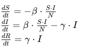
Here,
- is the number of susceptible individuals,
- is the number of infectious individuals,
- is the number of recovered individuals,
- is the total population,
- is the transmission rate, and
- is the recovery rate.
Let’s implement the SIR model in Python:
import numpy as np
from scipy.integrate import odeint
import matplotlib.pyplot as plt
# Function to define the SIR model equations
def sir_model(y, t, beta, gamma):
S, I, R = y
dSdt = -beta * S * I / N
dIdt = beta * S * I / N – gamma * I
dRdt = gamma * I
return [dSdt, dIdt, dRdt]
# Parameters
N = 1000 # Total population
I0 = 1 # Initial number of infectious individuals
R0 = 0 # Initial number of recovered individuals
S0 = N – I0 – R0 # Initial number of susceptible individuals
beta = 0.3 # Transmission rate
gamma = 0.1 # Recovery rate
# Time points
t = np.linspace(0, 200, 200)
# Initial conditions vector
y0 = [S0, I0, R0]
# Integrate the SIR equations over the time grid
solution = odeint(sir_model, y0, t, args=(beta, gamma))
# Plot the results
plt.plot(t, solution[:, 0], label=’Susceptible’)
plt.plot(t, solution[:, 1], label=’Infectious’)
plt.plot(t, solution[:, 2], label=’Recovered’)
plt.xlabel(‘Time’)
plt.ylabel(‘Population’)
plt.title(‘SIR Model Simulation’)
plt.legend()
plt.show()
This code uses the odeint function from the scipy library to solve the system of differential equations.
Extending to the SEIR Model
While the SIR model is effective, it does not account for the incubation period during which individuals are exposed to the virus but not yet infectious. The SEIR model addresses this limitation by introducing an “Exposed” compartment. The differential equations for the SEIR model are as follows:
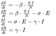
Here, represents the number of exposed individuals, and is the rate of transition from the exposed to the infectious state.
Let’s implement the SEIR model in Python:
# Function to define the SEIR model equations
def seir_model(y, t, beta, sigma, gamma):
S, E, I, R = y
dSdt = -beta * S * I / N
dEdt = beta * S * I / N – sigma * E
dIdt = sigma * E – gamma * I
dRdt = gamma * I
return [dSdt, dEdt, dIdt, dRdt]
# Parameters
sigma = 0.2 # Rate of transition from exposed to infectious state
# Initial conditions vector
y0_seir = [S0, I0, 0, R0] # No initially exposed individuals
# Integrate the SEIR equations over the time grid
solution_seir = odeint(seir_model, y0_seir, t, args=(beta, sigma, gamma))
# Plot the results
plt.plot(t, solution_seir[:, 0], label=’Susceptible’)
plt.plot(t, solution_seir[:, 1], label=’Exposed’)
plt.plot(t, solution_seir[:, 2], label=’Infectious’)
plt.plot(t, solution_seir[:, 3], label=’Recovered’)
plt.xlabel(‘Time’)
plt.ylabel(‘Population’)
plt.title(‘SEIR Model Simulation’)
plt.legend()
plt.show()
In this code, we’ve added an “Exposed” compartment to the state vector and modified the equations accordingly.
Analyzing the Results
After simulating the models, we can analyze the results to gain insights into the disease dynamics. Key factors include the peak of the infectious curve, the duration of the outbreak, and the effectiveness of interventions such as social distancing or vaccination campaigns.
# Find the peak of the infectious curve in the SIR model
peak_infectious_sir = np.max(solution[:, 1])
peak_infectious_sir_day = np.argmax(solution[:, 1])
print(f”SIR Model: Peak Infectious Cases = {int(peak_infectious_sir)}, Day = {peak_infectious_sir_day}”)
# Find the peak of the infectious curve in the SEIR model
peak_infectious_seir = np.max(solution_seir[:, 2])
peak_infectious_seir_day = np.argmax(solution_seir[:, 2])
print(f”SEIR Model: Peak Infectious Cases = {int(peak_infectious_seir)}, Day = {peak_infectious_seir_day}”)
This code snippet calculates and prints the peak infectious cases and the corresponding day for both models.
Conclusion
In this article, we’ve explored the implementation of two fundamental models for simulating infectious disease spread: the SIR and SEIR models. These models provide valuable insights into the dynamics of epidemics and play a crucial role in public health planning and decision-making. By employing Python and numerical integration techniques, we can simulate and analyze the spread of diseases, assess the impact of interventions, and make informed predictions about future outbreaks. These models serve as valuable tools for researchers, epidemiologists, and policymakers working to understand and mitigate the impact of infectious diseases on populations worldwide.